Essbase calculation engine - Black magic demystified

Introduction

In Essbase user’s world how a number is computed by the engine was a mystery all these years. In some simple to moderate cases it was possible to understand how and why a number was derived that way, but the more complicated the model the harder it was to understand what it is doing. This is not so surprising considering the nature of multi-dimensional modeling. Database designers used to wonder why is this number this instead of what they thought it would be. Sometimes they used to get surprised to see that nothing was calculated at all and it is returning #Missing. So every one used to call this “black magic” and did experiments to derive certain behaviors and blogged about it. The correct modeling was completed through trial and error or you can say try and cry if you want to be funny.

The Essbase team understood this and wanted to change this. We want to make this easy for the user. We introduced this feature called calculation tracing that will help you understand how a particular number was derived or why it was not calculated at all and is still #Missing.

Let me walk you through how you can use this. I am going to represent our model through our new innovation called the DBX workbook.

The Model

Let us say you have model with three dimensions Calendar, Product and Measures. They are shown below.

Now I loaded some data into ShippedUnits for products P1-a1, P1-a2,  P1-a3, P1-a4 for FY19 months (FY19-Jan, FY19-Feb so on and so forth). Similarly for P2-bx combinations and P3-cx combinations.

I also loaded ParentForecastUnits for P1-Clone, P2-Clone, P3-Clone for both FY19 months and FY20 months.

The calculation scrips

Now I wrote two calculation scripts one called shipped_percent.csc

And the next one called forecast.csc

Test and validate the numbers

Now I went to smart view and created the following query sheet. Note “-“ are all #Missing in these pictures.

Examine the query sheet. Products are listed in column A. P1-a1 and P1-clone are products. As you can see if you look at the Dim.Products sheet, both are children of P1, a product category.

Measures are named in column B of the query sheet. You can see details about them on the Dim.Measures sheet; for example, notice that ShippedPercentage and ParentForecastUnits do not consolidate.

Columns C:G on the query sheet are for fiscal year 2019, and columns H:L are for fiscal year 2020. In this exercise, assume we are in FY2019, trying to forecast for FY2020.

In C2:E2, data exists for units shipped in the first quarter of FY2019. Based on those initial numbers, we’ll do two calculations:

 a) C3:E3: the percentage of total shipped units (C10:E10) that is attributable to P1-a1 (for example, we expect that C3=C2/C10, or about 40%)

 b) H5:J5 -- a shipped-units forecast for the same quarter a year later. The allocations for FY2020 are based on the Shipped Percentage for the same product in FY2019. For example, we expect that H5=H8*C3, or about 18,261

Now Go to the Essbase ribbon, click Calculate, and run the shipped_percent calculation. Then run the forecast calculation also. Refresh the sheet. I am surprised. Cell C3 is not what I thought it would be. Its #Missing.

CALCTRACE to the rescue

Alright, let me see how I can use Calculation tracing to get some help. I went to the application configuration, and added a configuration setting CALCTRACE TRUE. Restarted the application.

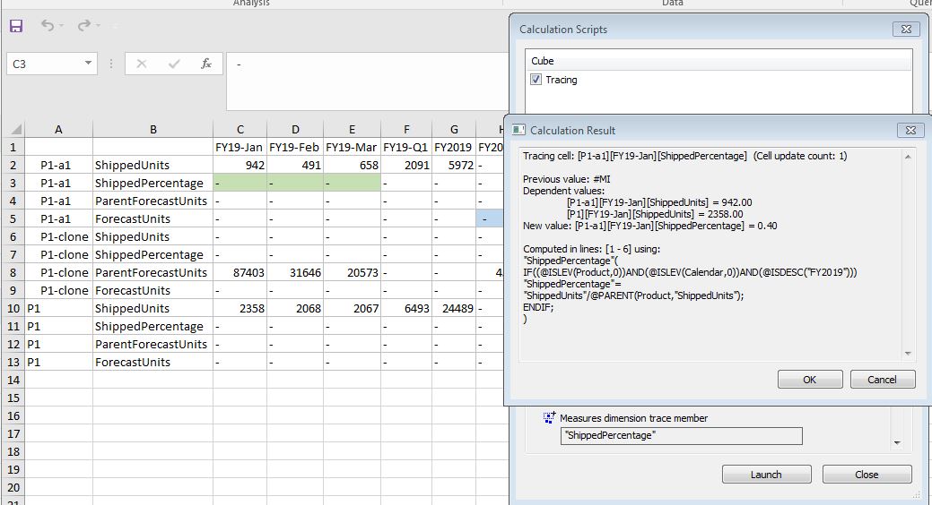
Then came back to query sheet and reconnected. Now I kept my mouse on cell C3 and ran shipped_precent calculation. Now the output shows me what happened.

Essbase displays the calculation tracing information, which shows you that cell C3 was not affected by the calculation. This usually means the cell is not in the calculation’s scope. Errors pertaining to scope often mean that you need to debug a FIX or IF statement.

I looked at my shipped_percent.csc. Ah! I got it. The error is in the IF statement. For a historical allocation for Jan-2019 to be in scope, the IF statement should reference 2019, not 2020. Correct, validate, and save the calculation.

Re-run the shipped percentage calculation, from cell C3, to compute C3:E3. Tracing information displays, showing you the effect the calculation had on C3. Refresh the sheet. The numbers should change for C3:E3 (C3 is approximately 0.399 or about 40%).

Execute the forecast script to get the right numbers for H5:J5 (Hint: H5 should be about 18,261).

To turn off calculation tracing when you don’t need it anymore, return to Essbase in your web browser. Select the application, launch the inspector, and click Configuration. Double click the ON value next to the CALCTRACE property, change it to OFF, and click Apply and Restart.

Conclusion

As you can see Calculation trace clearly helps with understanding a lot more about what is happening inside the Essbase engine.

Currently CALCTRACE should only be reliably used in application development phase. Meaning only one user should be running calculations on this database while you have this enabled for this to reliably show you what happened.

If you liked it, let us know. If you want to see more capabilities from this feature, let us know as well. 

Announcing Layouts, Reports and Impersonation in OAC - Essbase

In this post, I am going to explain what are the layouts, reports in the Essbase Analyze UI and how that will help the users to view and export the data in few clicks.

This feature is only introduced in the web UI but soon will be part of the SmartView as well.

Layouts
Layouts are nothing but the saved grids or bookmarked grids. SmartView is great and it allows to zoom in, zoom out and type to view the data required. When we work on the same or few grids again and again, every time launching SmartView and navigating by clicking ad-hoc buttons does not make any sense. It not only waste users time but also waste the resources on server to compute various operations.

Layouts are introduced to address this problem and save the grid as we go and navigate so that can be viewed anytime.

Reports
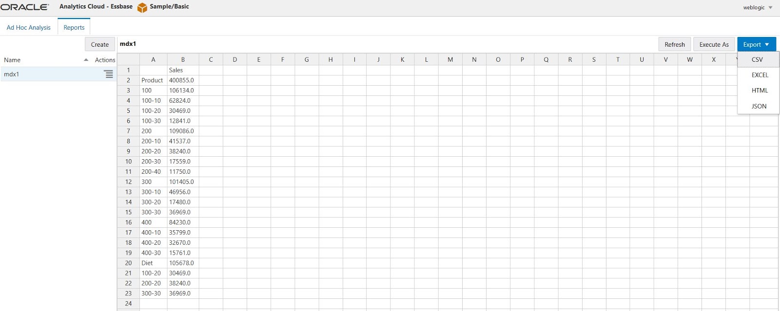
Reports are nothing but saved MDX queries but will be extended to data source queries as well. It would be interesting to join the MDX query with any relational or files data and view that to get what we need. For now, you can type the MDX queries and save them and run anytime. You can export the result into various formats as well like Excel, CSV, HTML and JSON.

You can run these reports as other user too just to make sure security filters are applied correctly on that user. You have to be system administrator to use impersonation.

Lets dive and see them in details:
1. Click on Analyze data on applications page - > Cube actions
2. You see the default grid.
3. Do some operations and close the browser tab.
4. repeat 1
5. Now you see the report you built in step #3. Its called session layout so system is smart enough to save your last navigated stuff.

If you are a DB manager, you can mark the layout as database default. Once you mark it, every user will see the same on launch unless they have their own default layout.

So algorithm is simple:
1. Looks for my default
2. if not #1, Looks for DB default
3. if not #2, Looks for Session
4. if not #3, Default grid

Here are the few screens:

All the REST apis can be impersonated provided that login user is System administrator.
Just add the X-Essbase-LoginAs header in REST call.

Sandbox and Scenario Workflow in Essbase for 1000's of users

In Essbase, one can always create a new dimension and clone the data and give to different users. This bloats the cube and doesnt scale to large number of users.  One needs to introduce strict limits on number of members in that sandbox/version/scenarion dimension. Also, since it is a metadata, business users cannot create new sandbox members.

We introduced new sandboxing and scenario management capabilities in Essbase in cloud. This is light weight and highly scalable and provides necessary isolation like Excel on your laptop for users. Moreover, end users can create new scenarios without involving admin.

Please watch the video for more details:

Essbase and light weight sandbox

Thanks
Kumar

Announcing Multi-Cell, Multi-Region Drill through

As we have seen in earlier blog posts, how easy it is to create a drill through reports in OAC - Essbase. If you have not read the earlier post yet then read it here.

In this post I am just focusing on multi-cell/multi region drill-through reports. Don't worry, there is no change required on your earlier reports. They will just keep working with single as well as multi selections.

Requirement:
You need latest SmartView for trying this out. If you need time to update SmartView on all your user machines then you can keep old SmartView and single cell based drill through will keep working as earlier.

Make sure that your instance is OAC 5.2 or later.

What is Multi-Cell :
Multi-Cell is when you select continuous cells in the Excel like B3, B4

What is Multi-Region:
Multi-Region is when you select multiple non continuous multi-cells. :)
In other words, when you select any number of regions(use ctrl+select to select multiple non-continuous ) you want in Excel.
e.g. It's very common for us to see the detailed report for all the months till September  excluding quarters like below.

Now go ahead and select such cells where drill through reports are defined and run drill through.

What should you expect when you click on drill through toolbar button:

Listing:
When you select multiple cells or regions, and there are multiple drill through reports, intersections of those reports are shown.
e.g. If you select A1, A2 and A3  and here is the cell to reports mapping
A1: R1
A2: R1, R3, R2
A3:  R1, R3, R4

then only R1 is common so it will be executed directly.

If you select only A2 and A3 then both R1 and R3 are listed. You can select one and then execute it.

Same will happen with multi region. Report(s) should be available for all the cells you selected.

Execution:
For Multi-Cell:
Think of it as running a SQL like select r1,r2,r3 where f1 in (a1,a2,a3) and f2 in (b1,b2,b3)
Where r1,r2 and r3 are the report columns and f1 and f2 are mapped columns for A and B dimension.

For single cell the query was like:
select r1,r2,r3 where f1=a1 and f2=b1

So only change is the replacement of equal operation with IN operation.

If you want sorted data etc then its better to define the data source query itself with sorting or use excel sorting once report is landed.

For Multi-Region:
Now think of it as running multiple SQL statements in parallel (one per region).
select r1,r2,r3 where f1 in (a1,a2,a3) and f2 in (b1,b2,b3)
+
select r1,r2,r3 where f1 in (i1,i2,i3) and f2 in (j1,j2,j3)
+
select r1,r2,r3 where f1 in (x1,x2,x3) and f2 in (y1,y2,y3)

As these queries are run in parallel and appended together in the result to improve the performance, data will remain unsorted. You can sort it in the Excel.

The combination of recursive, multi cell and multi region drill through is so fascinating! 

Try it out!

Autonomous Database support in Essbase

Happy New Year 2019!

In my earlier post, we learnt to use existing CLI to connect to ADW and ATP. This was just a workaround and new OAC-Essbase CLI does not need it anymore.

However the workaround was only for CLI and there was no support through UI and REST.
From OAC 5.2, Essbase CLI, UI and REST support to create connection to autonomous database(Autonomous data warehouse and transaction processing).

This post will demonstrate to create a connection to ADW and that connection can then be used to data load, build dimension, drill through or any other use cases using Essbase data sources abstraction.

Step 1. Download the wallet ZIP from your ADW/ATP instance.

Step 2. If you need any proxy settings to connect to the database then extract the zip, change/add proxy details in the tnsnames.ora. This is specified in the post I mentioned at the start of this post.

Step 3: Create an Oracle Database - Autonomous Connection like below:

Now create a data source and use it to load data, build a dimension, drill through ....

Rest :

To upload wallet file for a connection to be created called myconn:
curl "http://host/essbase/rest/v1/connections/myconn/wallet" -X PUT
-H "Content-type: application/octet-stream"
 --data <Wallet file path>

To create:
curl "http://host/essbase/rest/v1/connections" -H "Content-Type: application/json"
--data "{""name"":""myconn"",""description"":"""",""type"":""DB"",""service"":""essbaseadw"",""walletPath"":""/system/wallets/myconn"",""user"":""ADMIN"",""password"":""password""}"

Why Essbase?

Recently I had a chance to meet Jim Dorian and Bob Earle, the original founders of Essbase.  We met at the 25th birthday party for Essbase ... it has been 25 years since Arbor Soft went public.  This motivated me to produce this video to re-enforce the great features of Essbase, which is going very strong in cloud and on-premise and has a strong following among customers and partners.

I talk about the foundations needed in any Analytic Engine and why Essbase is well suited and best data structure for an analytic database. This talk could have been given 30 years back by the original founders.  We have been continuing to improve the aggregation and calculations capabilities and the scale at which we operate. Also, our focus has been on the cloud to provide this wonderful software on the cloud.

Please stay tuned for my next presentation coming soon which will talk about "20 reasons to consider Essbase in cloud".

Here is the link to the video of "Why Essbase?":

https://youtu.be/dw6dOSP9Jd8

Here are some pictures from 25th birthday party for Essbase:

Regards

Kumar

Loading Data from ADW/ATP to Essbase using CLI

Autonomous data ware house and transaction processing cloud provides a new way to connect and that will be adapted by many cloud vendors in coming releases. The new approach is more secure and wallet based.

In current version, OAC - Essbase does not support direct load from wallet based connections. This may come eventually in coming releases, this article will show a hack till that time. Even though there are ways to export to file and load that file to Essbase, CLI seems a better approach. As Essbase CLI gives you full control over the classpath, you can tweak it to suit your needs and support any JDBC.

In this article, we will see how we can achieve the dimension build or data load with CLI in minimal steps.

Estimated time to complete: 15 minutes

Download the ADW/ATP JDBC jars from OTN.

https://www.oracle.com/technetwork/database/application-development/jdbc/downloads/jdbc-ucp-183-5013470.html

Download the ojdbc8-full.tar.gz and extract it into CLI-INSTALL-DIR/lib

Replace the files on conflict.

Change the esscs.sh (Linux client) or esscs.bat (Windows client) to link the new jars.

CMD file changes (highlighted in green color)

set CLASSPATH=.;%REST_CLI_HOME%/ess_rest_cli.jar;%REST_CLI_HOME%/ess_es_server.jar;%REST_CLI_HOME%/ess_japi.jar;%REST_CLI_HOME%/ess_svp.jar;%REST_CLI_HOME%/commons-cli.jar;%REST_CLI_HOME%/commons-io.jar;%REST_CLI_HOME%/jersey-client.jar;%REST_CLI_HOME%/javax.ws.rs-api.jar;%REST_CLI_HOME%/jersey-common.jar;%REST_CLI_HOME%/hk2-utils.jar;%REST_CLI_HOME%/javax.inject.jar;%REST_CLI_HOME%/hk2-locator.jar;%REST_CLI_HOME%/hk2-api.jar;%REST_CLI_HOME%/javax-annotation-javax-annotation-api.jar;%REST_CLI_HOME%/jackson-annotations.jar;%REST_CLI_HOME%/jackson-core.jar;%REST_CLI_HOME%/jackson-databind.jar;%REST_CLI_HOME%/jackson-mapper-asl-1.9.2.jar;%REST_CLI_HOME%/ojdl.jar;%REST_CLI_HOME%/jersey-guava.jar;%REST_CLI_HOME%/cglib.jar;%REST_CLI_HOME%/jackson-core-asl-1.9.2.jar;%JAVA_HOME%/db/lib/derby.jar;%REST_CLI_HOME%/ojdbc8.jar;%REST_CLI_HOME%/ess-platform-common.jar;%REST_CLI_HOME%/commons-lang.jar;%REST_CLI_HOME%/datasource-model.jar;%REST_CLI_HOME%/excel-core.jar;%REST_CLI_HOME%/lz4-java.jar;%REST_CLI_HOME%/avatica-core.jar;%REST_CLI_HOME%/calcite-core.jar;%REST_CLI_HOME%/calcite-linq4j.jar;%REST_CLI_HOME%/protobuf-java.jar;%REST_CLI_HOME%/janino.jar;%REST_CLI_HOME%/commons-compiler.jar;%REST_CLI_HOME%/guava.jar;%REST_CLI_HOME%/slf4j-api.jar;%REST_CLI_HOME%/slf4j-nop.jar;%REST_CLI_HOME%/commons-lang3.jar;%REST_CLI_HOME%/ucp.jar;%REST_CLI_HOME%/ons.jar;%REST_CLI_HOME%/oraclepki.jar;%REST_CLI_HOME%/orai18n.jar;%REST_CLI_HOME%/osdt_cert.jar;%REST_CLI_HOME%/osdt_core.jar;%REST_CLI_HOME%/simplefan.jar;%REST_CLI_HOME%/xdb6.jar

Bash File changes (Highlighted in Green color)

export CLASSPATH=.:$REST_CLI_HOME/ess_rest_cli.jar:$REST_CLI_HOME/ess_es_server.jar:$REST_CLI_HOME/ess_japi.jar:$REST_CLI_HOME/ess_svp.jar:$REST_CLI_HOME/commons-cli.jar:$REST_CLI_HOME/commons-io.jar:$REST_CLI_HOME/jersey-client.jar:$REST_CLI_HOME/javax.ws.rs-api.jar:$REST_CLI_HOME/jersey-common.jar:$REST_CLI_HOME/hk2-utils.jar:$REST_CLI_HOME/hk2-apijar:$REST_CLI_HOME/javax.inject.jar:$REST_CLI_HOME/hk2-locator.jar:$REST_CLI_HOME/hk2-api.jar:$REST_CLI_HOME/javax-annotation-javax-annotation-api.jar:$REST_CLI_HOME/jackson-annotations.jar:$REST_CLI_HOME/jackson-core.jar:$REST_CLI_HOME/jackson-databind.jar:$REST_CLI_HOME/jackson-mapper-asl-1.9.2.jar:$REST_CLI_HOME/ojdl.jar:$REST_CLI_HOME/jersey-guava.jar:$REST_CLI_HOME/cglib.jar:$REST_CLI_HOME/jackson-core-asl-1.9.2.jar:$JAVA_HOME/db/lib/derby.jar:$REST_CLI_HOME/ojdbc8.jar:$REST_CLI_HOME/ess-platform-common.jar:$REST_CLI_HOME/commons-lang.jar:$REST_CLI_HOME/datasource-model.jar:$REST_CLI_HOME/excel-core.jar:$REST_CLI_HOME/lz4-java.jar:$REST_CLI_HOME/avatica-core.jar:$REST_CLI_HOME/calcite-core.jar:$REST_CLI_HOME/calcite-linq4j.jar:$REST_CLI_HOME/protobuf-java.jar:$REST_CLI_HOME/janino.jar:$REST_CLI_HOME/commons-compiler.jar:$REST_CLI_HOME/guava.jar:$REST_CLI_HOME/slf4j-api.jar:$REST_CLI_HOME/slf4j-nop.jar:$REST_CLI_HOME/commons-lang3.jar:$REST_CLI_HOME/ons.jar:$REST_CLI_HOME/oraclepki.jar:$REST_CLI_HOME/orai18n.jar:$REST_CLI_HOME/osdt_core.jar:$REST_CLI_HOME/osdt_cert.jar:$REST_CLI_HOME/simplefan.jar:$REST_CLI_HOME/ucp.jar:$REST_CLI_HOME/xdb6.jar

Extract the DB wallet file and store it in some path. I am going to use /scratch/wallets/adwwallet in this example.

Use the proxy (in tnsnames.ora) if your client machine is behind the firewall as per document: https://docs.oracle.com/en/cloud/paas/autonomous-data-warehouse-cloud/user/connect-preparing.html#GUID-EFAFA00E-54CC-47C7-8C71-E7868279EF3B

e.g.

ADWC1_high =

       (description=

             (address=

                   (https_proxy=proxyhostname)(https_proxy_port=80)(protocol=tcps)(port=1522)(host=adwc.example.oraclecloud.com)

             )

             (connect_data=(service_name=adwc1_high.adwc.oraclecloud.com)

             )

             (security=(ssl_server_cert_dn="adwc.example.oraclecloud.com,OU=Oracle BMCS US,O=Oracle Corporation,L=Redwood City,ST=California,C=US")

             )

       )

All set. Let’s try CLI commands now.

Make sure you have latest JDK 1.8.162+

$esscs.sh login -user weblogic -password welcome1 –url <OAC-ESSBASE-URL>

where OAC-ESSBASE-URL – https://essbase.example.oraclecloud.com/essbase

$esscs.sh createLocalConnection -name adwConn -connectionString  "jdbc:oracle:thin:@ adw_service_name?TNS_ADMIN=/scratch/wallets/adwwallet" -user adw_user -password adw_password

Pay attention to the new format of JDBC string.

To build a dimension:

$esscs.sh dimbuild -application Sample -db Basic -rule prod1m.rul -stream -restructureOption ALL_DATA -connection adwConn -query " SELECT PRODUCT, MARKET, ….  FROM TABLE WHERE …."

To load data:

$esscs.sh dataload -application Sample -db Basic -stream -connection adwConn -query "SELECT PRODUCT, MARKET, ….  FROM TABLE WHERE …." -rule prod1mdata.rul

Output:

Streaming to Essbase...

.............................................................................................................................................................................................

Streamed 1000005 rows to cube

And it works!

Make sure that your select query returns exactly same number of columns as specified in the rules file, otherwise Essbase will fail to load.